Efficient Attention Methods

Abstract

In modern transformers, the attention operation is the only component with a time complexity of $\mathcal{O}(N^2)$, whereas all other operations scale linearly as $\mathcal{O}(N)$, where $N$ denotes the sequence length. As sequence lengths in generative models (e.g., language and video generation) continue to increase, improving the efficiency of attention has become increasingly critical. Recently, numerous excellent works have been proposed to enhance the computational efficiency of attention operation. Broadly, these works can be classified into four categories: (1) Hardware-efficient attention: Optimizing attention computation efficiency by leveraging hardware characteristics. (2) Sparse attention: Selectively performing a subset of computations in attention while omitting others. (3) Compact attention: Compressing the KV cache of attention by weight sharing or low rank decomposition while keeping computational cost unchanged, as with a full‑sized KV cache. (4) Linear attention: Redesigning the computational formulation of attention to achieve $\mathcal{O}(N)$ time complexity. In this paper, we present a comprehensive survey of these efficient attention methods.

Overview

Efficient attention methods aim to reduce the time or memory costs of the standard attention mechanism. These approaches can be divided into four main categories:

Hardware-efficient attention: Optimizes the implementation by better utilizing modern GPU features like tiling and kernel fusion, without changing the attention logic.
Compact attention: Compresses the KV cache using techniques like weight sharing or low-rank decomposition to reduce memory overhead during inference.
Sparse attention: Reduces computational cost by skipping calculations for non-critical parts of the attention matrix, using either fixed or dynamic sparse masks.
Linear attention: Removes the softmax operation to reorder matrix multiplications, avoiding the O(N²) time complexity and reducing it to linear O(N).

Overview of four efficient attention methods — Figure 1: Overview of efficient attention methods.

1. Hardware-Efficient Attention

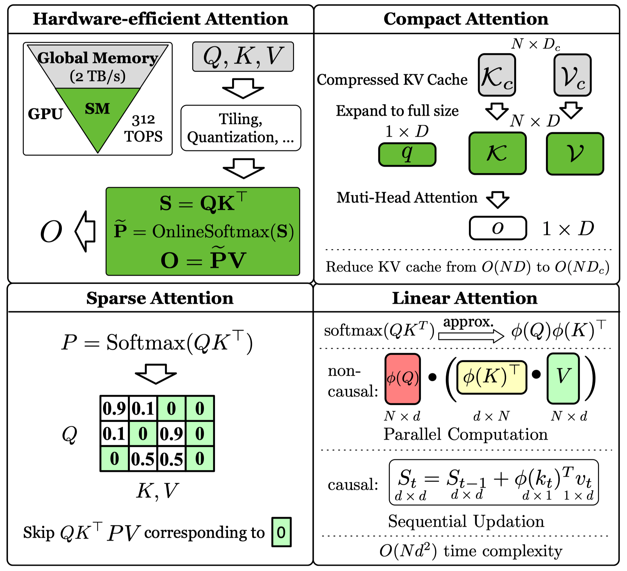
On modern GPUs, an operation's speed is limited by either computation (making it compute-bound) or memory data transfer (making it memory-bound). Hardware-efficient attention methods directly target these bottlenecks by optimizing how computations are performed and data is moved through the GPU's memory hierarchy.

Corresponding to the two stages in LLM inference (prefilling and decoding), Hardware-efficient Attention can be divided into two categories:

Prefilling methods, inspired by FlashAttention, partition $Q$, $K$, and $V$ into blocks $\mathbf{Q}_i$, $\mathbf{K}_i$, $\mathbf{V}_i$. They compute each output block $\mathbf{O}_i$ iteratively as follows:

$$ \hat{\mathbf{Q}}, \hat{\mathbf{K}}, \hat{\mathbf{V}} = \Psi(\mathbf{Q}), \Psi(\mathbf{K}), \Theta(\mathbf{V}). $$ $$ \mathbf{S} = \hat{\mathbf{Q}} \hat{\mathbf{K}}^\top, \quad \hat{\mathbf{P}} = \Theta (\mathrm{softmax}(\mathbf{S})), \quad \mathbf{O} = \hat{\mathbf{P}} \hat{\mathbf{V}}, $$

where $\Psi(\cdot), \Theta(\cdot)$ are preprocess functions to accelerate computation, e.g., quantization functions.

Decoding methods also partition $K$ and $V$ into blocks, but their input $\mathbf{q}$ is a vector, so the output vector $\mathbf{o}$ is computed as follows:

$$ \hat{\mathbf{K}}, \hat{\mathbf{V}} = \Psi(\mathbf{K}), \Theta(\mathbf{V}). $$ $$ \mathbf{s} = \mathbf{q} \hat{\mathbf{K}}^\top, \quad \mathbf{p} = \mathrm{softmax}(\mathbf{s}), \quad \mathbf{o} = \mathbf{p} \hat{\mathbf{V}}. $$

where $\Psi(\cdot), \Theta(\cdot)$ are KV cache preprocess functions.

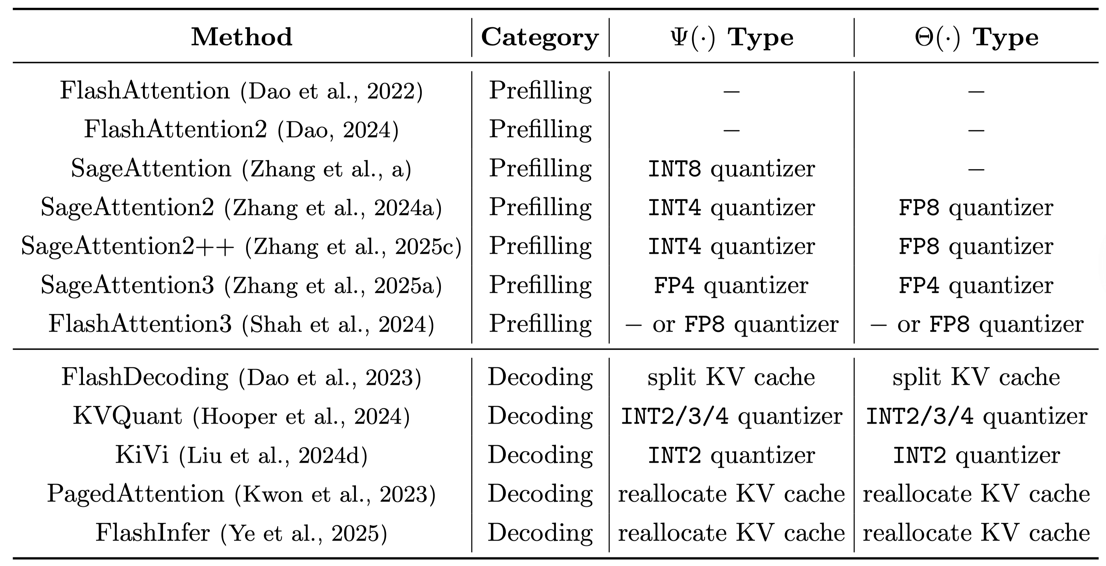
We summarize these hardware-efficient methods in Table 1. The $\Psi(\cdot)$ and $\Theta(\cdot)$ types refer to different pre-processing functions, such as splitting the KV cache across the GPU's SMs or reallocating it into efficient formats like pages (e.g., PagedAttention) to boost I/O speed.

2. Compact Attention

Compact attention methods are designed to reduce the memory consumption of the KV cache during LLM inference. In MHA, we store the full-resolution KV matrices exactly as used in computation, causing the KV cache size to grow rapidly. Compact attention methods decouple storage KV from computation KV, storing compressed KV states and expanding them for computation. This approach significantly reduces storage KV size compared to MHA, lowering memory usage, while preserving the computation KV size to prevent significant performance degradation.

The general formulation can be expressed as follows.

$$ \begin{align} q, \mathcal{K}_c, \mathcal{V}_c &= \text{proj}_\mathcal{Q}(x), \text{proj}_{\mathcal{K}_c}(X), \text{proj}_{\mathcal{V}_c}(X). \\ \mathcal{K}, \mathcal{V} &= \text{expand}_\mathcal{K}({\mathcal{K}_c}), \text{expand}_\mathcal{V}({\mathcal{V}_c}). \\ o &= \text{MHA}(q, \mathcal{K}, \mathcal{V}). \end{align} $$

where $\mathcal{K} = [K^{(1)}, \dots, K^{(h)}] \in \mathbb{R}^{N \times D}$ denotes the concatenation of $h$ attention head key matrices, with $K^{(i)} \in \mathbb{R}^{N \times d}$ representing the key matrix of head $i$ and $D = h d$. The same notation applies to $q$ and $\mathcal{V}$. Here, $x \in \mathbb{R}^{D_m}$ is the hidden state of the current token, $X \in \mathbb{R}^{n \times D_m}$ is the matrix of hidden states for the context tokens, $\text{proj}(\cdot)$ and $\text{expand}(\cdot)$ denote the projection and expansion functions, respectively, and $\text{MHA}(\cdot)$ denotes the multi-head attention operation.

We summarize the KV cache size for each token, total parameters for attention, and expansion function type for compact attention methods in Table 2.

3. Sparse Attention

The attention map $P = \mathrm{Softmax}(QK^\top / \sqrt{d})$ exhibits inherent sparsity, as the softmax operation often creates many values approaching zero. Sparse attention methods exploit such sparsity to accelerate attention by two steps. First, it constructs a sparse mask $M$, which determines whether to compute or skip specific elements in the attention map $P$. Second, it computes attention only for the parts corresponding to the sparse mask $M$.

$$ \begin{align} P &= \mathrm{Softmax}(M + QK^\top / \sqrt{d}). \\ O &= PV. \end{align} $$

Where $M$ is an $N \times N$ matrix whose elements are either 0 or $-\infty$. $M_{i,j} = 0$ specifies that both the attention score $Q_iK_j^T$ and its corresponding output $P_{i,j}V_j$ should be computed, while $M_{i,j} = -\infty$ indicates these computations should be skipped.

There are two distinct categories of sparse attention methods based on how the sparse mask is generated:

Pattern-based method relies on predefined sparsity patterns derived from empirical observations, where the positions of $-\infty$ entries in $M$ follow fixed geometric shapes (e.g., a sliding window shape).
Dynamic sparse attention computes the sparse mask $M$ adaptively during runtime based on some input-dependent functions (e.g., $M_{i,j} = -\infty$ if $\mathrm{pool}(Q_i) \mathrm{pool}(K_j^T) < \tau$ for a threshold $\tau$, where $\mathrm{pool}(\cdot)$ could be mean pooling over tokens).

We summarize sparse attention methods based on their sparse mask $M$ (pattern-based or dynamic), whether it can reduce KV cache storage, whether they need to train a model, and applicability to language models and diffusion transformers in Table 3.

4. Linear Attention

Linear attention methods reduce the computational complexity from $O(N^2)$ to $O(N)$ by replacing the softmax function with a kernel function. This allows for a reordering of matrix multiplications, avoiding the explicit computation of the N×N attention matrix. For autoregressive tasks, these methods can be formulated in a recurrent manner, using a fixed-size state that is updated at each step. This makes them highly efficient for inference on very long sequences.

Naive Formulation

$$ \begin{aligned} H_t &= H_{t-1} + \phi(k_t)^\top v_t \\ o_t &= \phi(q_t)H_t \end{aligned} $$

Computation Forms

Figure 2 shows three computation forms of linear attention.

Linear Parallel Form. This form calculates the output $O$, using $O=\phi(Q)(\phi(K)^\top V)$, by computing the $\phi(K)^T V$ first, the computational complexity is decreased to $O(Nd^2)$. It is highly efficient for the training and inference of non-autoregressive (NAR) tasks, where the entire sequence is processed simultaneously. For autoregressive training, forcing causality with a mask $O = (\phi(Q) \phi(K)^\top \odot M)V$.

Recurrent Form. This form introduces a fixed-size state $H_t$ that is updated recurrently: $H_t = H_{t-1} + \phi(k_t)^\top v_t$. The output is then computed as $o_t=\phi(q_t)H_t$. When computing, it first computes the $\phi(k_t)^T v_t$ and then updates the hidden state $H_t$, finally compute $o_t=\phi(q_t)H_t$.

Chunk-wise Form. This form is a hybrid solution designed for autoregressive training, resolving the issues of the previous forms. It divides the sequence into fixed-size chunks and uses a dual strategy: Attention is computed in quadratic parallel form within each chunk to maximize parallelization. Causality is maintained by passing a recurrent state between chunks. As the figure shows, the final attention output for each chunk is the sum of two distinct components:

Intra-chunk Attention: This part is computed using standard, parallel masked self-attention on the Query, Key, and Value matrices within the current chunk. It captures local dependencies inside the chunk.
Inter-chunk Attention: This part incorporates historical information from all previous chunks. It is computed by combining the current chunk's Query with the hidden state passed from the prior chunk.

Four Categories of Linear Attention

To enable the fixed-size hidden state $H_t$ to dynamically hold the most relevant information, the forget and select gates were introduced. Then the $H_t$ update can be formulated as: $$ H_t = G_f^{(t)} \odot H_{t-1} + G_s^{(t)} \odot \phi(k_t)^\top v_t. $$ $G_f^{(t)} $ acts as a forget gate, deciding how much historical information ($H_{t-1}$) to keep, and $G_s^{(t)}$ serves as a select gate, determining how much current information to hold. The computation can be shown as Figure 3.

Linear Attention with Gates — Figure 3: Linear attention with forget and select gates.

Linear attention methods can be classified by their hidden state update method. The first three categories rely on direct computation of $H_t$:

(1) Naive Linear Attention: Linear attention without gates, i.e., both $G_f^{(t)}$ and $G_s^{(t)}$ are fixed as $\mathbf{1}^\top \mathbf{1}$, Table 4 shows some typical naive linear attention methods.

Table 4: Summary of naive linear attention methods.
(2) Linear Attention with a Forget Gate: Only $G_s^{(t)}$ is fixed as $\mathbf{1}^\top \mathbf{1}$, while the forget gate $G_f^{(t)}$ is predefined or input-dependent, Table 5 shows some typical linear attention methods with a forget gate. All the complexities shown in the table are the complexities of the training phase.

Table 5: Summary of linear attention with forget gate only.
(3) Linear Attention with both Forget and Select Gates: both $G_f^{(t)}$ and $G_s^{(t)}$ are predefined or input-dependent rather than fixed as $\mathbf{1}^\top \mathbf{1}$. Table 6 shows some typical linear attention methods with forget and select gates. All complexities shown in the table are the complexities of the training phase.

Table 6: Summary of linear attention methods with forget and select gates.

Test-Time Training

Test-Time Training (TTT) views the hidden state $H_t$ as a set of learnable parameters, also called `fast weights'. TTT continuously update the hidden state via gradient descent during both training and inference. This can be shown as Figure 4. This hidden states update process is different with the first three categories of linear attention methods, thus we categorize it as the fourth category of linear attention in the paper.

For the full paper, please see our paper.

BibTeX


        @article{zhang2025efficient,
          title={A Survey of Efficient Attention Methods: Hardware-efficient, Sparse, Compact, and Linear Attention},
          author={Zhang, Jintao and Su, Rundong and Liu, Chunyu and Wei, Jia and Wang, Ziteng and Zhang, Pengle and Wang, Haoxu and Jiang, Huiqiang and Huang, Haofeng and Xiang, Chendong and Xi, Haocheng and Yang, Shuo and Li, Xingyang and Hu, Yuezhou and Fu, Tianyu and Zhao, Tianchen and Zhang, Yicheng and Cao, Boqun and Jiang, Youhe and Chen, Chang and Jiang, Kai and Chen, Huayu and Zhao, Min and Xu, Xiaoming and Wu, Yi and Bao, Fan and Zhu, Jun and Chen, Jianfei},
          year={2025}
        }